Keynesianism

Key assumption:

• Wages and prices are “rigid” or “sticky” and do not adjust quickly to market-clearing levels
• Business cycles are primarily caused by shocks to the aggregate demand

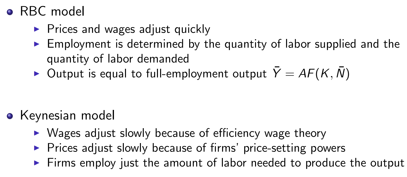
• Wages adjust slowly because of efficiency wage theory
• Prices adjust slowly because of firms’ price-setting powers
• Firms employ just the amount of labor needed to produce the output

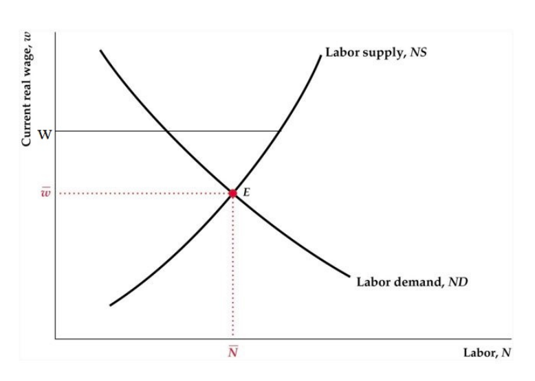
Wage Rigidity

real wage moves too little to equate $N^s$ and $N^d$

$⟹$ Efficiency wage model

Higher wage $⟹$ desire to keep job $\uparrow ⟹$ effort $\uparrow$

Higher wage $⟹$ employer-employee relations $\uparrow ⟹$ effort $\uparrow$

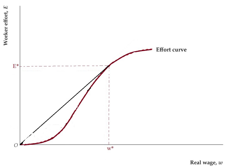
$w^{\ast }$ at tangency point maximizes $\frac{E}{w}$ or effort per dollar paid

given $w$ the firm chooses $N^d$ based on $w=\text{MPN}$

Unemployment

if $w^{\ast }>w_E$ unemployment occurs

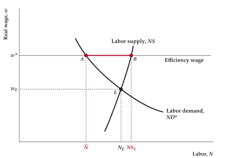
Unemployment given by difference in $\bar{N}$ (A) and $N^s$ (B) at efficiency wage level ($w^{\ast }$)

During recessions $N^d\downarrow$ so $\bar{N}\downarrow ⟹$ Unemployment $(N^s-\bar{N})\uparrow$

Empirically real wage is procyclical

• effort changes in recessions

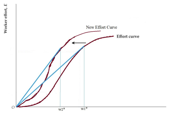
People work harder because they are more concerned about losing their jobs

Employment depends on $N^d$ not $N^S$ if efficiency wage > market clearing wage

Price Rigidity

In perfectly comp firms are price takers

• P = MC

In monopolistic comp firms set prices w/ markup

• P > MC

there are costs to changing prices (menu costs) empirically most firms do not change prices frequently

Effective Labor Demand Curve

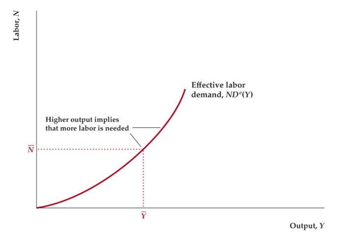
Firms choose labor based on output

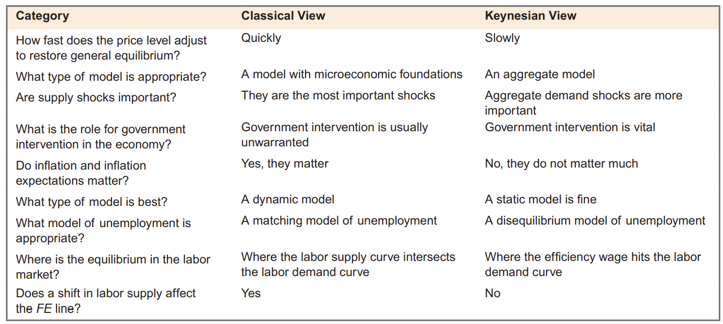
Summary of Differences

Labor Productivity

• The fact that average labor productivity is empirically procyclical is not explained by Keynesian model

adjustment with utilization

average labor productivity may fall during recessions if labor is utilized less intensively $U_N\downarrow ⟹\frac{Y}{N}\downarrow$

Monetary Policy

GIVEN $M^S\uparrow$:

Variable	RBC (no misperception)	Keynesian (SR)	Keynesian (LR)
Y	-	$\uparrow$	-
$r$	-	$\uparrow$	-
C	-	$\uparrow$	-
I	-	$\uparrow$	-
N	-	$\uparrow$	-
P	$\uparrow$	-	$\uparrow$

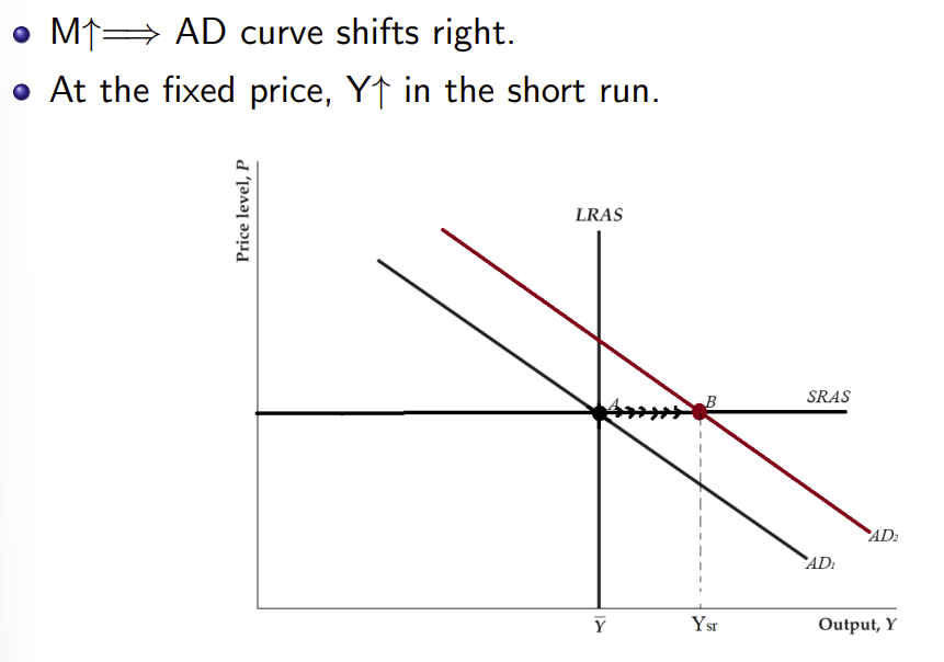
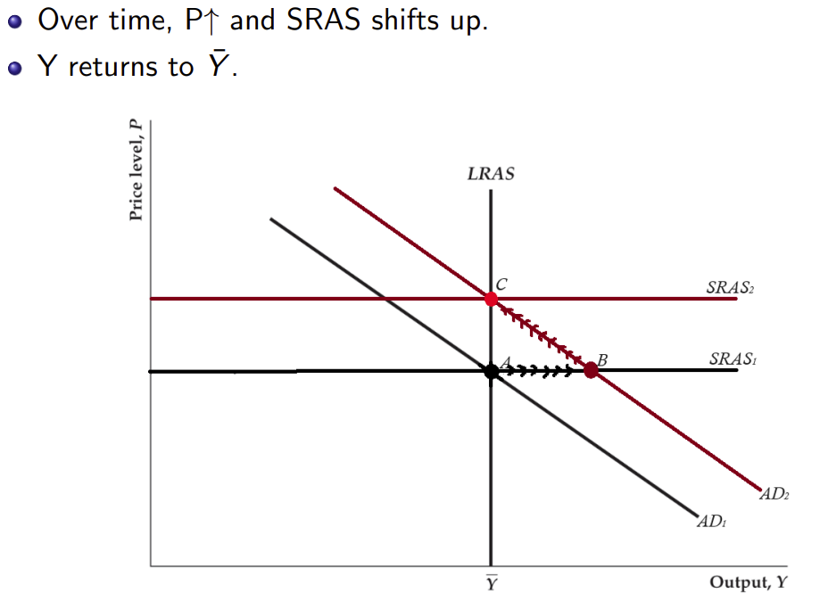
Monetary Policy not neutral in SR

• menu costs → firms don’t react to increased demand by raising prices, instead increase production to meet higher demand
• $Y>\bar{Y}$ temporarily

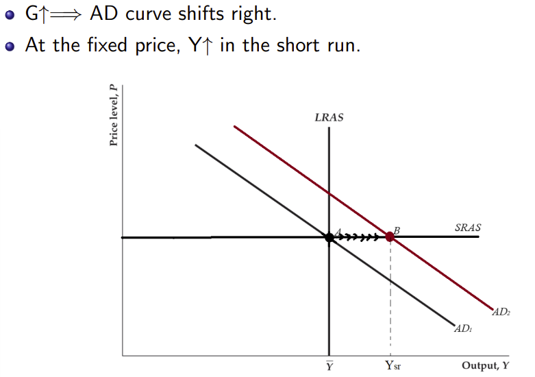
Fiscal Policy

GIVEN $G\uparrow$:

Variable	RBC (no misperception)	Keynesian (SR)
$\bar{Y}$	$\uparrow$	-
Y	$\uparrow$	$\uparrow$
$r$	$\uparrow$	$\uparrow$
N	$\uparrow$	$\uparrow$
P	$\uparrow$	-

Government Spending Multiplier

• The SR change in Y from a one-unit change in G
• Multiplier = $\frac{\Delta Y}{\Delta G}$
• Keynesians argue it is greater than 1
  • $G\uparrow$ raises income of consumers so $C\uparrow$
  • $\Delta Y=\Delta C+\Delta G⟹\frac{\Delta Y}{\Delta G}>1$

Lump Sum Tax-Cut

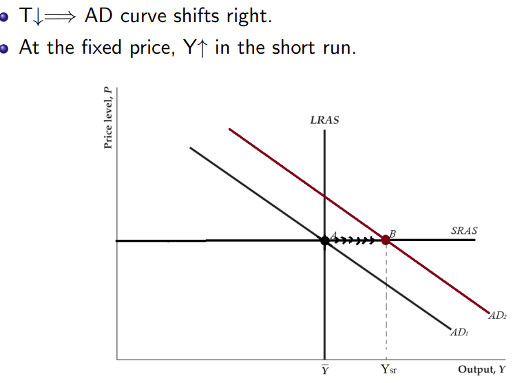
Government Spending multiplier not present here instead it is the tax multiplier which may not be greater than 1

• When G ↑, ∆Y = ∆C + ∆G
• When T ↓, ∆Y = ∆C

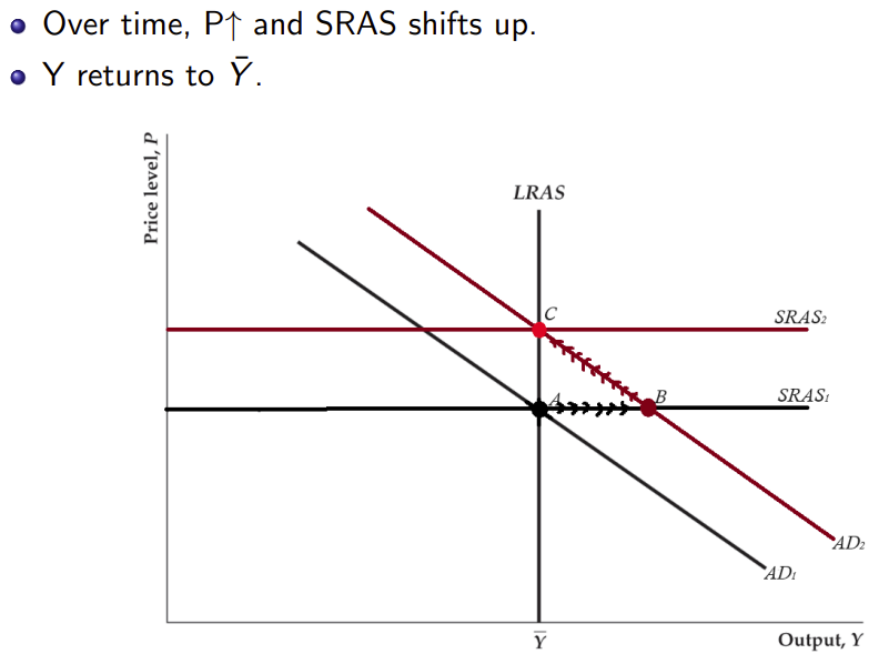
Summary

• In the Keynesian model, G ↑ or T ↓ will increase Y in SR
• Y deviates from the full-employment output due to an increase in aggregate demand
• The government spending multiplier is greater than the tax multiplier

Macroeconomic Stabilization and Demand shocks

• Do nothing: economy corrects itself but possibly slow price adjustment process, output and employment remain below their full-employment levels.
• $M^s$ ↑: LM shifts to the right and the economy could return to general equilibrium faster
• G ↑: IS shifts to the right and the economy could return to general equilibrium faster